The Normal Distribution & Visualizer

In this tutorial, we will explore the Normal Distribution, a fundamental concept in statistics.

The following topics will be covered in this tutorial:

A probability distribution is a combination of a variable and its corresponding probabilities of each value. The Normal Distribution, known as the bell curve, is one of the most significant statistical distributions in use today. Its typical nature is explained in the following diagram:

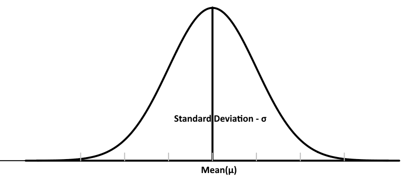
Most human characteristics, such as height, weight, waist-size, blood pressure, etc., follow a normal distribution. The mean of the distribution is located at the center of the curve, while the standard deviation determines the spread of the data. The area under the curve represents the total probability, which is equal to 1 that makes it a probability distribution.
The normal distribution is widely used in various fields, including statistics, finance, and social sciences, to model real-world phenomena and make predictions based on data.

The smaller the standard deviation, the narrower and taller the bell curve will be, indicating that the data points are closely clustered around the mean. On the other hand, a larger standard deviation results in a wider and flatter curve, suggesting that the data points are more spread out from the mean. The normal distribution is also characterized by its symmetry around the mean, meaning that the left and right sides of the curve are mirror images of each other. This property allows for various statistical analyses and hypothesis testing to be conducted using the normal distribution as a reference point.
In addition, mode and median are also located at the center of the curve, which means that in a normal distribution, the mean, median, and mode are all equal. This is a unique property of the normal distribution and contributes to its widespread use in statistical analysis.

Properties of the Normal Distribution

• 💎 Mean, Median, and Mode: In a normal distribution, the mean, median, and mode are all equal and located at the center of the curve.
• 💎 Symmetry: The normal distribution is symmetric around the mean, meaning that the left and right sides of the curve are mirror images of each other.
• 💎 68-95-99.7 Rule: Approximately 68% of the data falls within one standard deviation of the mean, 95% within two standard deviations, and 99.7% within three standard deviations.

With the following simulation, you can visualize the normal distribution: choose your value of standard deviation and mean with the sliders below and adjust the size of the variable to see the area under the curve.

 

Worked Examples

E.g.1

The diameters of a nail produced by a particular machine, Xmm, are modelled as X~N(6, 0.5). Find:
a) P(X > 6)
b) P(5.5 < X <6.5)
c) P(X < 5.5)
d) P(X > 7)
e) P(5 < X < 7)

a) P(X > 6) = 0.5
b) P(5.5 < X < 6.5) = 0.6827
c) P(X < 5.5) = 0.1587
d) P(X > 7) = 0.0228
e) P(5 < X < 7) = 0.9545

E.g.2

The arm spans of a group of teenagers in a gymnastic club, Xcm, are modelled as X ~ N(120, 9).
a State the proportion of students who have an arm span between 117 cm and 123 cm.
b State the proportion of students who have an arm span between 114 cm and 126 cm.

1. a) P(117 < X < 123) = 0.68 (approx — using the 68% rule, ±1σ)
2. b) P(114 < X < 126) = 0.95 (approx — using the 95% rule, ±2σ)

E.g.3

The lengths of a group of cats, X cm, are modelled as X ~ N(30, σ²). If 68% of the cats have a length between 23 cm and 37 cm, find the variance, σ2.

Using the 68% rule (≈ mean ± 1σ): the interval 23 to 37 is 30 ± σ, so σ = 7. Therefore the variance is σ² = 49.

E.g.4

The weights of a group of dogs, X kg, are modelled as X ~ N(20, σ²). If 95% of the dogs have a weight between 10 kg and 30 kg, find the variance, σ2.

Using the 95% rule (≈ mean ±2σ): the interval 10 to 30 is 20 ± 2σ, so σ = 5. Therefore the variance is σ² = 25.

E.g.5

The weights of a group of squirrels , Q grams, are modelled as Q ~ N(μ, 5²). If 97.5% of the squirrels weigh less than 120 grams, find the mean.

Using the 97.5% rule (≈ mean + 2σ): the interval is Q < 120, so 120 = μ + 2(5) → μ = 110 grams. Due to the symmetry of the bell curve. The area of the two extremes are 2.5% each, that leaves the area of the central section at 95%.

E.g.6

The masses of a herd of cows, M kg, on a farm are modelled as M ~ N(μ, σ²). If 84% of the cows weigh more than 180 kg and 97.5% of the cows weigh more than 160 kg, find µ and σ.

Using the 68% rule: about 16% lies below μ − σ. Here 84% weigh more than 180 kg, so 16% weigh ≤ 180 kg → 180 ≈ μ − σ.

Using the 95% rule: about 2.5% lies below μ − 2σ. Here 97.5% weigh more than 160 kg, so 2.5% weigh ≤ 160 kg → 160 ≈ μ − 2σ.

Solve the two equations: μ − σ = 180 and μ − 2σ = 160. Subtracting gives σ = 20 kg, then μ = 200 kg standard deviation = 20 kg.

Standard Normal Distribution

The standard normal distribution is a special case of the normal distribution where the mean (μ) is 0 and the standard deviation (σ) is 1. It is often denoted as Z ~ N(0, 1) and the process of converting a normal random variable to a standard normal random variable is called standardization. The values of the standard normal distribution are called z-scores.

Standardized scores or z-scores are widely used in real life situations. z-scores are used in determining how many people will be qualified for a particular program based on their test scores.

E.g.

In Sri Lanka, the island in the Indian Ocean, z-scores are used to determine university admission eligibility based on student performance. A few weeks after the A Level results are announced, students' z-scores are calculated to assess their relative performance.

Why do we standardize? Standardizing allows us to use a single table (the z-table) to find probabilities for any normal distribution, regardless of its mean and standard deviation. Although we have calculators to find probabilities of normal distributions today in 2026 for any value of mean and standard deviation, it was not the case about 20 years ago. There was only one table those days for finding probabilities of the normal distribution. That table is for the standard normal distribution, which simplifies the process and makes it more efficient.

In order to use this specific table, we need to convert our normal random variable, X, to a standard normal random variable, Z, using the formula:
Z = (X - μ) / σ.

X ~ N(μ, σ²) → Z ~ N(0, 1)

In the above animation, you can see how normal distributions with different means and standard deviations that raise the need for standardization - using a single z-table.

The standard normal distribution table looks like this:

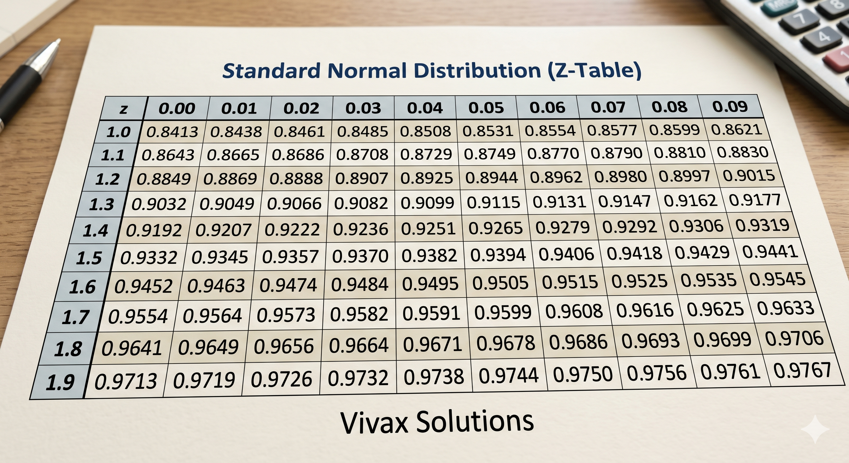
Now, let's see how to use the z-table to find probabilities.

E.g.1

The weight of a certain type of fruit is normally distributed with a mean of 100 grams and a standard deviation of 10 grams. Find the probability that a randomly selected fruit weighs less than 110 grams.

X ~ N(100, 10²)

Find P(X < 110).

Standardize: Z = (X - μ) / σ = (110 - 100) / 10 = 1

P(X < 110) = P(Z < 1) = 0.8413 ← from the z-table or calculator

E.g.2

The height of a certain type of plant is normally distributed with a mean of 50 cm and a standard deviation of 5 cm. Find the probability that a randomly selected plant is taller than 55 cm.

X ~ N(50, 5²)

Find P(X > 55).

Standardize: Z = (X - μ) / σ = (55 - 50) / 5 = 1

P(X > 55) = P(Z > 1) = 1 - P(Z < 1) = 1 - 0.8413 = 0.1587
Note: P(Z > 1) = 1 - P(Z < 1) because the total area under the curve is 1, so the area to the right of Z = 1 is the complement of the area to the left of Z = 1.

E.g.3

The lifespan of a certain type of light bulb is normally distributed with a mean of 1000 hours and a standard deviation of 50 hours. Find the probability that a randomly selected light bulb lasts between 700 and 1100 hours.

X ~ N(1000, 50²)

Find P(700 < X < 1100).

Standardize: Z = (X - μ) / σ = (700 - 1000) / 50 = -6 and Z = (1100 - 1000) / 50 = 2

P(700 < X < 1100) = P(-6 < Z < 2) = P(Z < 2) - P(Z < -6) = 0.9772 - 0.0000 = 0.9772

E.g.4

The scores of a certain type of exam are normally distributed with a mean of 75 and a standard deviation of 8. Find the probability that a randomly selected student scores between 65 and 72.

X ~ N(75, 8²)

Find P(65 < X < 72).

Standardize: Z = (X - μ) / σ = (65 - 75) / 8 = -1.25 and Z = (72 - 75) / 8 = -0.375

P(65 < X < 72) = P(-1.25 < Z < -0.375) = P(Z < -0.375) - P(Z < -1.25) = 0.3531 - 0.1056 = 0.2475

E.g.5

The heights of a certain type of tree are normally distributed with a mean of 10 meters and a standard deviation of 2 meters. Find the probability that a randomly selected tree is between 8 and 12 meters tall.

X ~ N(10, 2²)

Find P(8 < X < 12).

Standardize: Z = (X - μ) / σ = (8 - 10) / 2 = -1 and Z = (12 - 10) / 2 = 1

P(8 < X < 12) = P(-1 < Z < 1) = P(Z < 1) - P(Z < -1) = 0.8413 - 0.1587 = 0.6826

⬇️ Inverse Standard Normal Distribution

P(Z < z) can also be written as Φ(z), where Φ is the cumulative distribution function of the standard normal distribution. That means that if we have a probability value, we can find the corresponding z-score using the inverse of the cumulative distribution function, denoted as Φ^-1(p). This is useful for finding z-scores corresponding to specific probabilities.

E.g.1

Find the z-score such that P(Z < z) = 0.95.

We need to find z such that Φ(z) = 0.95. Using the z-table or a calculator, we find that z ≈ 1.645.

E.g.2

Find the z-score such that P(Z < z) = 0.025.

We need to find z such that Φ(z) = 0.025. Using the z-table or a calculator, we find that z ≈ -1.96.

E.g.3

Find the z-score such that P(Z < z) = 0.5.

We need to find z such that Φ(z) = 0.5. Using the z-table or a calculator, we find that z ≈ 0.

E.g.4

Find the z-score such that P(Z < z) = 0.975.

We need to find z such that Φ(z) = 0.975. Using the z-table or a calculator, we find that z ≈ 1.96.

E.g.5

Find the z-score such that P(Z < z) = 0.05.

We need to find z such that Φ(z) = 0.05. Using the z-table or a calculator, we find that z ≈ -1.645.

E.g.6

Find the z-score such that P(Z < z) = 0.995.

We need to find z such that Φ(z) = 0.995. Using the z-table or a calculator, we find that z ≈ 2.576.

⬇️ Finding Quartiles and Percentiles of the Standard Normal Distribution

The first quartile (Q1) is the z-score such that P(Z < Q1) = 0.25, the second quartile (Q2) is the z-score such that P(Z < Q2) = 0.5, and the third quartile (Q3) is the z-score such that P(Z < Q3) = 0.75.

E.g.1

Find the first quartile (Q1) of the standard normal distribution.

We need to find Q1 such that P(Z < Q1) = 0.25. Using the z-table or a calculator, we find that Q1 ≈ -0.674.

E.g.2

Find the second quartile (Q2) of the standard normal distribution.

We need to find Q2 such that P(Z < Q2) = 0.5. Using the z-table or a calculator, we find that Q2 ≈ 0.

E.g.3

Find the third quartile (Q3) of the standard normal distribution.

We need to find Q3 such that P(Z < Q3) = 0.75. Using the z-table or a calculator, we find that Q3 ≈ 0.674.

E.g.4

Find the 90^th percentile of the standard normal distribution.

We need to find z such that P(Z < z) = 0.90. Using the z-table or a calculator, we find that z ≈ 1.282.

E.g.5

Find the 10^th percentile of the standard normal distribution.

We need to find z such that P(Z < z) = 0.10. Using the z-table or a calculator, we find that z ≈ -1.282.

E.g.6

Find the 99^th percentile of the standard normal distribution.

We need to find z such that P(Z < z) = 0.99. Using the z-table or a calculator, we find that z ≈ 2.326.

⬇️ Finding the mean and standard deviation of a Normal Distribution

Given a normal distribution with mean μ and standard deviation σ, we can find the mean and standard deviation using the z-scores corresponding to specific probabilities.

E.g.1

Given that P(X < 110) = 0.8413 for a normal distribution X ~ N(100, σ²), find the standard deviation (σ).

Standardize: Z = (X - μ) / σ = (110 - 100) / σ = 10 / σ

P(X < 110) = P(Z < 10 / σ) = 0.8413

Using the z-table or a calculator, we find that 10 / σ ≈ 1, so σ ≈ 10.

E.g.2

Given that P(X > 55) = 0.1587 for a normal distribution X ~ N(µ, 5²), find the mean (µ).

Standardize: Z = (X - μ) / σ = (55 - µ) / 5

P(X > 55) = P(Z > (55 - µ) / 5) = 0.1587

Using the z-table or a calculator, we find that (55 - µ) / 5 ≈ 1, so µ ≈ 50.

E.g.3

Given that P(90 < X < 110) = 0.6826 for a normal distribution X ~ N(100, σ²), find the standard deviation (σ).

Standardize: Z = (X - μ) / σ = (90 - 100) / σ = -10 / σ and Z = (110 - 100) / σ = 10 / σ

P(90 < X < 110) = P(-10 / σ < Z < 10 / σ) = 0.6826

Using the z-table or a calculator, we find that -10 / σ ≈ -1 and 10 / σ ≈ 1, so σ ≈ 10.

E.g.4

Given that P(X < 85) = 0.0228 and P(X > 115) = 0.0228 for a normal distribution X ~ N(µ, σ²), find the mean and standard deviation (σ).

Standardize: Z = (X - μ) / σ = (85 - µ) / σ

P(X < 85) = P(Z < (85 - µ) / σ) = 0.0228

Using the z-table or a calculator, we find that (85 - µ) / σ ≈ -2, so 85 - µ ≈ -2σ → µ ≈ 85 + 2σ.

Now we need another equation to solve for µ and σ. We can use the fact that P(X > 115) = 0.0228, which means P(X < 115) = 0.9772.

Standardize: Z = (X - μ) / σ = (115 - µ) / σ

P(X < 115) = P(Z < (115 - µ) / σ) = 0.9772

Using the z-table or a calculator, we find that (115 - µ) / σ ≈ 2, so 115 - µ ≈ 2σ → µ ≈ 115 - 2σ.

Now we have two equations: µ ≈ 85 + 2σ and µ ≈ 115 - 2σ. Solving these gives us 85 + 2σ ≈ 115 - 2σ → 4σ ≈ 30 → σ ≈ 7.5. Then µ ≈ 85 + 2(7.5) ≈ 100.

E.g.5

Given that P(X < 120) = 0.975 and P(X > 150) = 0.0025 for a normal distribution X ~ N(µ, σ²), find the mean and standard deviation (σ).

Standardize: Z = (X - μ) / σ = (120 - µ) / σ

P(X < 120) = P(Z < (120 - µ) / σ) = 0.975

Using the z-table or a calculator, we find that (120 - µ) / σ ≈ 1.96, so 120 - µ ≈ 1.96σ → µ ≈ 120 - 1.96σ.

Now we need another equation to solve for µ and σ. We can use the fact that P(X > 150) = 0.0025, which means P(X < 150) = 0.9975.

Standardize: Z = (X - μ) / σ = (150 - µ) / σ

P(X < 150) = P(Z < (150 - µ) / σ) = 0.9975

Using the z-table or a calculator, we find that (150 - µ) / σ ≈ 2.81, so 150 - µ ≈ 2.81σ → µ ≈ 150 - 2.81σ.

Now we have two equations: µ ≈ 120 - 1.96σ and µ ≈ 150 - 2.81σ. Solving these gives us 120 - 1.96σ ≈ 150 - 2.81σ → 0.85σ ≈ 30 → σ ≈ 35.29. Then µ ≈ 120 - 1.96(35.29) ≈ 50.

⬇️ Finding the conditional probability using the standard normal distribution

To find the conditional probability P(A | B), we use the formula:

P(A | B) = P(A ∩ B) / P(B)

For a normal distribution, this can be calculated using the standard normal distribution table or a calculator.

E.g.1

Given that P(X < 110) = 0.8413 and P(X > 90) = 0.1587 for a normal distribution X ~ N(100, 5²), find the conditional probability P(X < 110 | X > 90), using the standard normal distribution.

P(X < 110 | X > 90) = P(X < 110 ∩ X > 90) / P(X > 90)

P(X < 110 ∩ X > 90) = P(90 < X < 110) = P(X < 110) - P(X < 90) = P(Z < 2) - P(Z < -2) = 0.9772 - 0.0228 = 0.9544

P(X > 90) = P(Z > -2) = 0.9772

P(X < 110 | X > 90) = 0.9544 / 0.9772 ≈ 0.9767

E.g.2

Given that P(X < 120) = 0.975 and P(X > 100) = 0.1587 for a normal distribution X ~ N(110, 10²), find the conditional probability P(X < 120 | X > 100), using the standard normal distribution.

P(X < 120 | X > 100) = P(X < 120 ∩ X > 100) / P(X > 100)

P(X < 120 ∩ X > 100) = P(100 < X < 120) = P(X < 120) - P(X < 100) = P(Z < 1) - P(Z < -1) = 0.8413 - 0.1587 = 0.6826

P(X > 100) = P(Z > -1) = 0.8413

P(X < 120 | X > 100) = 0.6826 / 0.8413 ≈ 0.8115